2.0 LOLA INSTRUMENT DESCRIPTION AND FUNCTIONAL BLOCK DIAGRAM

The LOLA instrument configuration with the LOLA coordinate system is shown in Figure 2‑1 and Figure 2‑2, and the key instrument parameters are shown in Table 2‑1. LOLA uses a Q-switched Nd:YAG laser at 1064 nm and avalanche photo diodes (APD) to measure the time of flight (TOF) to the lunar surface from a nominal 50 km orbit. The transmitted laser beam is split in five different beams by a diffractive optical element (DOE) with 0.5 mrad spacing. The receiver telescope focuses the reflected beams into a fiber optic array, placed at the focal plane of the telescope. The array consists of five fibers. Each fiber in the array is aligned with a laser spot on the ground. The fibers direct the reflected beams into five detectors.

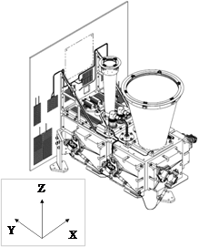
Figure 2‑1 LOLA Instrument configuration and coordinate system

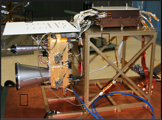
Figure 2‑2LOLA Instrument during testing

The detector electronics amplify the signal and then compare it against a pre-set threshold. The output of the comparators is then time stamped relative to the spacecraft mission elapsed time (MET) using a set of time-to-digital converters (TDCs) with 0.5 ns resolution. Both the rising and falling edges of the output of the comparators are recorded. Onboard algorithms filter out the false alarms and select the most likely ground echoes. The range gate limits the number of false alarms by detecting pulses arriving only within the expected time interval (the range to the surface). A noise counter records the numbers of threshold crossings at the output of each comparator and a detection threshold level is adjusted automatically such that the average number of false alarm pulses within the range gate interval is maintained at a predetermined value. The signal-processing algorithm also adjusts the receiver gain and maintains the range window centered on the lunar surface return.

The transmitted pulse is also time stamped and the TOF to the lunar surface can be determined. The LRO spacecraft carries an ultra-stable oven-controlled crystal oscillator that distributes the timing signal to LOLA and other instruments. A simplified functional block diagram of LOLA is shown in Figure 2‑3.

Table 2‑1 LOLA instrument parameters

Parameter	Value
Laser Wavelength	1064.4 nm
Pulse Energy	2.7-3.2 mJ
Pulse Width (FWHM)	~ 5 ns
Pulse Rate	28 ± 0.1 Hz
Beam Divergence	100 ± 10 mrad
Beam Separation	500 ± 20 mrad
Receiver Aperture Diameter	0.14 m
Receiver Field of View	400 ± 20 mrad
Receiver Bandpass Filter	0.8 nm
Detector responsivity (nominal)	300 kV/W
Detector active area diameter	0.7 mm
Detector electrical bandwidth	46 ± 5 MHz
Timing Resolution	0.5 ns

Riris_Fig2.tif

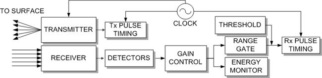
Figure 2‑3 LOLA functional block diagram

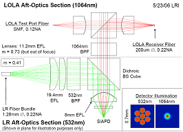
The LRO spacecraft also carries a unique laser ranging system for precise orbit determination. The laser ranging system consists of a 30 mm aperture optical receiver mounted on the LRO spacecraft high gain antenna used for communications and data transmitting. The receiver is pointed to a ground (earth) based laser satellite ranging station that sends a 532 nm laser pulse to LRO. The receiver focuses the incoming 532 nm beam into a fiber bundle and the laser pulses are then directed onto one of the five LOLA detectors modified to accommodate both 532 and 1064 signals. The timing of the ground-based laser is adjustable and is intended to arrive at LOLA well before the lunar returns.

2.1 LOLA TRANSMITTER

The LOLA transmitter consists of two virtually identical, diode pumped, Q-switched Nd:YAG oscillators operating at 1064.4 nm (Figure 2‑4).

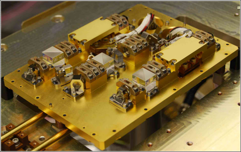
Figure 2‑4 LOLA laser transmitter

The diode pump lasers are derated to increase their lifetime. The laser beams are combined with polarizing optics and only one laser is operating at a time; the other one is redundant. The laser repetition rate is 28 ± 0.1 Hz, the energy per pulse is ~ 2.7 mJ for laser 1 and ~ 3.2 mJ for laser 2. The pulse width is approximately 5 ns. The output of the laser is directed through a ´18 beam expander and then through a diffractive optical element that produces five beams separated by 500 ± 20 mrad. The laser beam prior to the beam expander has a divergence of 1.8 mrad. After the beam expander and the diffractive optical element, each beam has a 100 ± 10 mrad divergence and approximately the same energy; some variation in the energy between beams is discernible due to imperfections in the diffractive optical element. The LOLA laser is designed to operate in vacuum but a significant amount of the sub-system and system testing was done in air. The laser cavity was integrated in a clean room and two filters in the laser housing are designed to prevent particulate and molecular contamination of the laser topics prior to launch.

The laser beam pattern is clocked at 26^o relative to the spacecraft velocity vector. From the nominal orbit of 50 km, each laser spot is approximately 5 m in diameter on the ground. The five spot pattern will allow LOLA to measure both the slope and the roughness of the lunar surface. The five beam spot pattern on the ground (including the field of view) relative to the spacecraft velocity vector is shown in Figure 2‑5.

A small kick-off mirror placed inside the laser box directs a small fraction of the laser power onto a silicon detector. The detector monitors the energy of the transmitted laser pulse and it also used as a fire acquisition signal that turns off the drive to the pump diode lasers. In addition, the outgoing pulse is time tagged and provides timing information for the time of flight measurement.

LOLA Spots.jpg

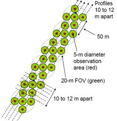
Figure 2‑5 LOLA five spot pattern

2.2 LOLA RECEIVER

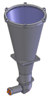
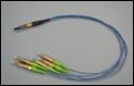
The LOLA receiver consists of a 14 cm clear aperture refractive telescope that focuses the received photons on to a fiber optic bundle. The effective focal length of the telescope is 500 mm. The design and materials of the telescope were chosen to minimize the thermal fluctuations expected on orbit. Since LOLA is not an imaging system, the objective is not to maintain the image quality but to collect the maximum number of photons with the fewest possible losses and to minimize the background radiation. The telescope assembly includes a dielectric fold mirror, which lets all radiation other than 1064 nm pass through and reflects the laser radiation on the fiber optic bundle. This minimizes the amount of background solar radiation incident on the detectors. The fiber bundle consists of five identical fibers. Each fiber in the bundle directs the reflected energy into the aft-optics assembly for each detector.

Figure 2‑6 LOLA receiver telescope

Figure 2‑7 LOLA receiver fiber bundle (EM)

The aft optics assemblies for detectors (channels) 2-5 are identical. Detector 1 houses the laser ranging aft optics. The aft-optics assembly mounts directly on a flange that is an integral part of the detector housing assembly. The housing assembly or detector plate includes the detector and all the associated electronics.

The aft optics consists of collimating and focusing optics to collimate the output of the fiber and send it on to the detector. A bandpass filter tuned to the laser wavelength at 1064.45 nm is also included in the optical train for each detector to minimize the background solar radiation. Detector 1 also includes a 532 nm bandpass filter for the laser ranging channel. In addition, the aft optics assembly for each detector includes a separate test port with an FC connector. The test port is intended for calibration purposes during instrument integration and testing. Signals from optical test sources can be injected into the test port and exercise the signal processing algorithms and electronics of the instrument. It is also possible to back-illuminate the detectors through the test port and monitor the field of view (FOV) and boresight alignment during the integration process. The detailed optical design for the LOLA detectors can be found in Ramos et.al. Optical system design and integration of the Lunar Orbiter Laser Altimeter, Applied Optics, Vol. 48, No. 16 / 3035, 2009.


Figure 2‑8 LOLA aft-optics detectors 2-5	Figure 2‑9 LOLA aft-optics detector 1

2.3 LOLA DETECTORS

The LOLA detectors are part of the detector housing assembly. The housing assembly includes the aft optics, the detector hybrid and the LOLA detector board (Figure 2‑10). The detectors and detector board electronics have low noise and sufficient bandwidth to allow detection of the reflected laser pulses from the lunar surface and measure the time of flight (TOF). Each detector has its own independent gain control and threshold setting. The detector hybrids are the same silicon avalanche photodiodes that were used on the Mars Orbiter Laser Altimeter (MOLA) [Smith et.al. 2002, Abshire et.al. 1999] and the Geoscience Laser Altimeter (GLAS) [Abshire et.al. 2005, Zwaly et.al. 2002]. The detectors are packaged in a hermetically sealed package with an integrated transimpedance amplifier.

The LOLA detector board amplifies the detector hybrid output, and performs two separate functions:

· a discrimination function to provide timing information to the Digital Unit (DU),

· an energy measurement function that integrates and samples the peak of the amplified hybrid output.

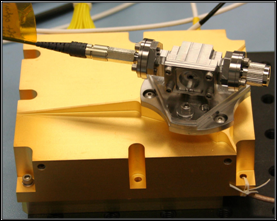
Figure 2‑10 LOLA detector

The amplification of the hybrid output is performed by a variable gain amplifier (VGA) and a fixed gain buffer with a gain of 5. The VGA gain is variable over a range of <0.5 to 10, controlled by an externally generated d.c. voltage from the DU. The gain control voltage is scaled and level-shifted on the detector board. The discrimination function for the timing information is performed by a high speed comparator. The threshold level is set by the DU and fed directly to the comparator input. The comparator output is intended to drive a 50-ohm load to ≥3 volts. There is an Enable input to shut down the comparator’s output in the event anything happens that would cause the channel to generate excessive noise counts.

The energy measurement function is performed by an integrator and a peak detector. It is not dependent on the threshold set by the DU but it is affected by the gain setting. The integrator stage is combined with a track-and-hold function which is controlled by a latch. The latch is set by a peak detector, and later reset by a signal from the DU. The peak detector responds to the integrator output so as to set the latch at the time of the maximum output from the integrator. The latch then puts the integrator into its HOLD mode until its output is digitized. The peak detector is an A.C.-coupled, D.C. offset constant-fraction discriminator. The output is proportional to the received energy.

2.4 LOLA DIGITAL UNIT

The LOLA Digital Unit is an integrated unit providing two fundamental categories of functionality for the instrument. The first category - range measurement - includes firing the laser and acquiring Earth and Lunar ranging data; the other category – command and telemetry (C&T) - comprises receiving and distributing spacecraft commands, collecting, formatting and transmitting telemetry, as well as monitoring and processing ranging information for real-time control of the altimeter’s parameters such as the range gate, amplifier gain and detector threshold.

2.4.1 Range Measurement Electronics

The implementation of range measurement functionality builds upon the techniques developed in previous planetary altimeters. Two different time measurements are made. The primary task is to “time-stamp” the laser transmit pulse and the five lunar return pulses, and the lunar ranging pulse.

The timing reference is based on a redundant 20 MHz ultra stable oscillator (USO) located in the spacecraft, which is divided down to 5 MHz and used as the internal timing reference. The spacecraft provides a non-redundant 1 Hz pulse, which is used to synchronize all LOLA activities. The fault-tolerant design allows for the spacecraft timing signals to replace the function of the internal clock oscillator, while the internal oscillator is sufficient to operate the instrument in the absence of any spacecraft timing reference. Also, circuits use the spacecraft’s ultrastable oscillator to measure the frequency of the on-card oscillator, for purposes of calibration and trending.

LOLA operates at pulse repetition frequency (PRF) of 28 Hz, phase locked to the spacecraft’s 1 Hz timing signal. Each 1 s interval is referred to as a major frame, which consists of 28 approximately 35.7 ms periods referred to as a minor frames, which begin at a time designated as T0. The time within a minor frame is allocated for various functions, which include an 8 ms window for receiving the Earth laser signal, a window for receiving the reflections from the Moon, and time for transmitting science and engineering data to the Command and Telemetry Electronics. The Range Measurement Electronics also synchronize the operation of the Analog Electronics and control the resetting of the energy measurement circuits for Detector boards (Figure 2‑11 LOLA Digital Unit timing diagram.

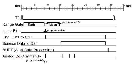
Figure 2‑11 LOLA Digital Unit timing diagram

The Range Measurement Electronics control is implemented in a single RTAX2000S Field Programmable Gate Array (FPGA). This FPGA also contains a variety of counters which implement the 200 ns coarse timer for each channel, noise counters, event counters, and calibration counters for measuring the margin in the digital phase lock loops in each of the twelve fine timing microcircuits.

There are six physical channels in the Range Measurement Electronics. One channel is utilized for the timing laser firing pulse, and the other five are for the lunar return pulses, with one of the return channels also time-shared for the earth laser time measurement. The time measurement method utilizes coarse timer implemented in FPGA along with fine timing supplied by digital ASIC time to digital converter (TDC) originally designed to support the ESA’s Automated Transfer Vehicle (ATD). The FPGA and TDC circuits together allow for time-tagging over planetary distances of the time that the laser is fired, the time the Earth-based laser’s signal arrives at the spacecraft, and the time of each of 5 returns received from the lunar surface.

IMG_0465small

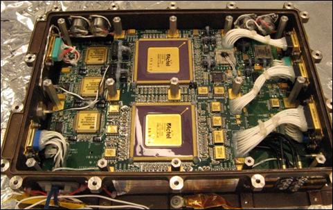
Figure 2‑12 LOLA digital unit

2.4.2 Command and Telemetry Electronics

The Command and Telemetry Electronics implement communications with the spacecraft, command and data distribution to other LOLA electronics, and the receipt of science data and telemetry both from the Range Measurement and the Analog Electronics. The Command and Telemetry Electronics are primarily implemented in two RTAX2000S FPGAs.

One FPGA known as the “RodChip” implements a MIL-STD-1553B dual-redundant Remote Terminal. Along with the required functions, the RodChip contains memory for loopback testing ensuring reliable communications, a discrete output register to control key instrument attributes such as laser selection, laser on/off, thermal electric cooler enables, and the write protection of critical memories. The RodChip also acts as a DMA controller, providing simple access to effectively all of the Digital Unit’s memory and registers.

The second FPGA provides hardwired command and telemetry functions. Commands are distributed as appropriate to the Analog Electronics and Range Measurement Electronics and received science and engineering data is formatted and stored in one of two telemetry buffers, which are read out by the spacecraft in 1 Hz intervals, for each major frame.

The second FPGA also provides the real-time function of determining the range gate, amplifier gains, and threshold voltages. This function is provided by a high-performance instruction set compatible version of an HS-80C85RH CPU implemented inside the FPGA. The CPU runs out of dual-redundant high-reliability radiation-hardened SRAM, which is loadable either from PROM, one of 4 pages of EEPROM, or directly from the ground. The entire software is less than 16 kbytes. For testing, calibration, and fault-tolerance, the CPU may be bypassed with all values supplied by ground command.

2.5 LOLA TIMING

The timing of LOLA is derived from the LRO Ultra-stable Oscillator (USO). LRO uses two USOs, each with two outputs, operating at 20 MHz. The outputs drive the Mission Elapsed Time (MET) and the timing of the LOLA DU timing. There are no USOs in the LOLA instrument.

LRO employs Coordinated Universal Time (UTC) to correlate spacecraft Mission Elapsed Time (MET) to ground time with an accuracy of ±3 ms. The clock frequency drift is estimated to be 3.5×10^-8/day, which satisfies the LOLA altimetry stability requirement (1×10^-7). In addition, the clock needs to be stable to < 2.0×10^-12/day (two parts per trillion stability) over the expected environmental temperature ranges to meet the laser ranging (LR) requirements. The drift and stability requirements require the use of oven controlled crystal oscillators (OCXO) which keep the crystal at a near constant temperature.

The timing sequence of major LOLA events is illustrated in Figure 2‑13. LOLA operates at a pulse repetition rate of 28 Hz (35.71 ms) which is phase locked to the spacecraft’s 1 Hz timing signal (1 pps). The earth range gate for laser ranging is triggered at T₀ and lasts about 8 ms (green traces in Figure 2‑13). The laser ranging signal must occur in this range gate. Only detector 1 has a laser ranging channel. The lunar range gate for all detectors is triggered by the LOLA Fire Command. The range gate is adjustable from 0 to 5 ms (~ 0-750 km) after the Fire Command. The laser fire occurs approximately 9.66 ms after T₀ (this includes the adjustable 150-210 us diode laser drive pulse). The Range Measurement Electronics time stamp the laser firing pulse (from the SPOT4 detector), and the five lunar return pulses (from the Rx detectors). They also provide a noise count which is used by the signal processing software to set the threshold crossings for all detectors.

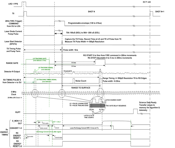
Figure 2‑13 LOLA timing diagram

3.0 LOLA LASER POINTING ANGLE AND LRO COORDINATE SYSTEM

The LOLA coordinate system is shown in Figure 3‑1. All the LOLA angular directions are referenced to the alignment reference cube attached to the side of the OTA as shown in Figure 3‑1. LOLA points in the +z direction (nadir) during normal operation.

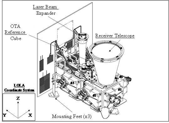
Figure 3‑1 LOLA coordinate system

The LOLA laser pointing relative to each channel in the OTA reference cube coordinate system was measured at the system level and verified in instrument TVAC. The results of these measurements are shown in Table 3‑1 and the spot pattern relative to the s/c x-axis is illustrated in Figure 3‑4.

Table 3‑1 LOLA pointing relative to OTA cube

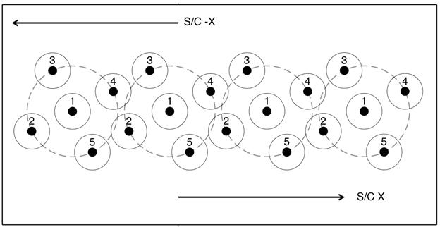
Figure 3‑2 LOLA pointing relative to OTA cube

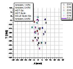
It is useful to transform the pointing measurements in Table 3‑1 (which are referenced to the OTA cube) to pointing measurements relative to Channel 1. This transformation enables us to better visualize the relative pointing of the four channels (relative to the channel 1). The results of this transformation are shown in Figure 3‑3. Figure 3‑3 also shows the arrangement of the detector layout relative to the x, y coordinates.

Figure 3‑3 Transformation of LOLA pointing measurements (relative to OTA cube), to measurements relative to Channel 1.

During instrument TVAC testing the LOLA laser pointing angle for all five beams was measured by imaging the beam with an off-axis parabola (OAP) along with a reference beam from the OTA reference cube onto a camera and measuring the angular offset between the laser images and the OAP optical axis. A GSE cube was also mounted on the TVAC fixture used to hold LOLA in the TVAC chamber to simulate the LRO reference cube and determine the LOLA-LRO pointing.

The results of the laser pointing angle for channel 1 relative to other four channels (beams) and the OTA reference cube over all temperatures are shown in Table 3‑2. There was very little change in the pointing relative to the OTA reference cube over the entire temperature range for both lasers (approximately 24 mrad for laser 1 and 23 mrad maximum excursion for laser 2).

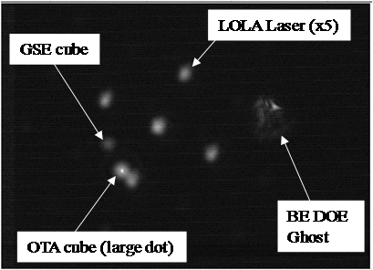
Figure 3‑4 LOLA pointing measurement image

Table 3‑2 LOLA laser pointing angle results during instrument TVAC

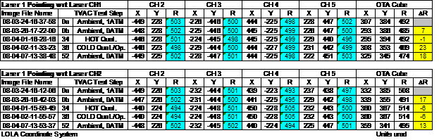
Table 3‑2 also lists the beam separation (channel spacing) over the entire instrument temperature range (~ 500 rad). The beam separation varies by less than 5 mrad over the entire temperature range which is within the measurement accuracy of the instrumentation.

The results of the LOLA pointing relative to the GSE cube (which were expected to simulate the LOLA – LRO pointing over temperature) were inconclusive. Unfortunately the GSE cube exhibited very large temperature fluctuations which distorted the pointing data, rendering them useless.

After integration to the spacecraft, the coordinates of the LOLA reference cube relative to the LRO alignment reference cube in the spacecraft coordinate system were surveyed and tracked during the spacecraft integration and testing process. (Note that the LOLA laser pointing measurements were not repeated at the spacecraft level but merely transferred from the LOLA coordinate system to the LRO coordinate system). The detailed alignment specification, verification, and survey history of LRO can be found in LRO-431-SPEC-000113 and LRO-451-RPT-003412. Here we will only summarize the final results after LRO had been shippd to the launch site.

The LRO spacecraft coordinate system (Body Coordinate System or BCS frame) along with the LRO instruments is shown in Figure 3‑5. The LRO coordinate axes point in the same direction as in the LOLA coordinate system with +z being the nadir direction, and +x being the direction of the spacecraft velocity. The LOLA reference cube measurements relative to the LRO alignment reference cube are shown in Table 3‑3 and the LRO master cube to the BCS frame are shown in Table 3‑4.

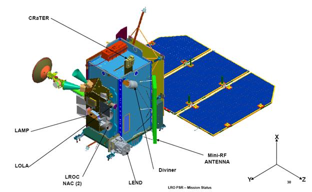
Figure 3‑5 LRO coordinate system

Table 3‑3 LOLA Cube to LRO Master Cube Transformation Matrix

	Roll	Yaw	Pitch
X	0.99999177	0.00381296	0.00138773
Y	-0.0037536	0.99917066	-0.0405452
Z	-0.0015412	0.04053961	0.99917674

Table 3‑4 LRO Master Cube to BCS frame Transformation Matrix

	Roll	Yaw	Pitch
X	0.99999177	0.00381296	0.00138773
Y	-0.0037536	0.99917066	-0.0405452
Z	-0.0015412	0.04053961	0.99917674

The transformation of the LOLA cube to the BCS frame is done by multiplying the matrices in Table 3‑3 and

Table 3‑4. The result is shown in Table 3‑5.

Table 3‑5 LOLA Cube to BCS frame Transformation Matrix

	Roll	Yaw	Pitch
X	0.99998757	0.00477017	0.00145188
Y	-0.0047642	0.99998032	-0.0040808
Z	-0.0014713	0.00407379	0.99999062

The most useful transformation in geo-locating the LOLA spots on the lunar surface is the measurements of the LOLA laser pointing in the BCS frame. Those measurements can be found in Table 3‑6 below.

Table 3‑6 LOLA Laser Channels in BCS frame Transformation Matrix

	Roll	Yaw	Pitch
Laser Ch1	0.001533728	-0.004489989	0.999988744
Laser Ch2	0.001315711	-0.004945780	0.999986904
Laser Ch 3	0.001994370	-0.004703150	0.999986951
Laser Ch 4	0.001761442	-0.004039041	0.999990292
Laser Ch 5	0.001087631	-0.004281670	0.999990242

The LOLA laser pointing relative to the star trackers was also measured during the LRO survey. The LOLA pointing was verified during the initial calibration of the instrument during flight. The procedures are listed in the LRO Instrument Calibration Specification 431-SPEC-002967.

4.0 LOLA RANGING (TOF) CALIBRATION

The primary function of LOLA is to provide time of flight (TOF) or altimetry measurements of the laser pulse which, along with the spacecraft position, can be used for determining the topography of the lunar surface. The LOLA TOF is determined by the following measurements: the Tx laser pulse leading edge time stamp (LET_x), the Tx laser pulse trailing edge time stamp (TET_x), the Rx laser pulse leading edge time stamp (LER_x), and the Rx laser pulse trailing edge time stamp (TER_x). The distance from the LRO spacecraft to an illuminated spot on the lunar surface, D, is related to the laser-pulse TOF by:

where c= 299792458 m/s is the speed of light in vacuum, and Tx and Rx are the times of the transmitted and echo laser-pulses. If the pulse shapes were perfectly symmetric, the pulse arrival times are simply taken as the average value of the signal threshold crossing times at the leading and trailing edges,

The distance traveled by the laser pulse and the spacecraft orbit position and pointing angle at the moment the laser-pulse was transmitted defines a vector in space which can be used to solve for the coordinates and the height of the laser footprint on a planet's surface given the position of the planet center of mass. A topographic map of the planet can be constructed with a great number of such measurements along different ground tracks. For a perfectly symmetric Gaussian pulse waveform, the leading and trailing edge points also provide a measurement of the Tx and Rx pulsewidth, if we also have knowledge of the laser energy.

4.1 CONVERTING LOLA TOF TO RANGE

In an ideal altimeter where the pulses would be perfectly symmetric and there would be no inherent biases in the time of flight (range) calculation. Of course, LOLA is not an ideal altimeter and we need to correct for several biases which are different for each detector. These corrections can be divided in two broad categories.

1. Fixed offsets (delays) due to the electronics (TDC trailing edge bias, different cable lengths), and delays due to the different fiber and cable lengths for each channel.

2. Variable offsets mainly due to the impulse response of the detector electronics which make the pulses asymmetric and introduce a range bias (or “time walk”) that is a function of the received signal amplitude.

4.1.1 Fixed Offsets

Rx fixed delays are listed below. Leading edge (LE) delays are relative to transmit LE, and trailing edge (TE) delays are relative to respective LE. Note that each TDC Phase has a different delay):

Channel	Fiber path delay t_fiber (ns)	Coax Cable delay	t_{off_chLE_ns}		t_{off_chTE_ns}
	Fiber path delay t_fiber (ns)	t_cable (ns)	Phase A	Phase B	Phase A	Phase B
TX	-		0.00	0.20	2.22	1.83
1	3.22	4.04	0.00	0.00	1.83	1.71
2	3.14	3.34	-0.30	-0.60	1.89	1.83
3	2.47	2.89	-0.50	-0.40	1.77	1.38
4	1.79	1.99	-2.10	-2.20	1.56	1.50
5	2.40	2.54	-1.20	-1.60	1.86	2.04

With

RX_nMID = (((t_rxTE-t_{off_rxnTE_ns})+t_rxLE)/2) - t_{off_rxnLE ns} - t_fiber– t_cable

and

t_rxLE = 200*RX_{n_coarse}- (RX_{n_fine3}-RX_{n_fine1})*0.02815;

t_rxTE = 200*RX_{n_coarse}- (RX_{n_fine3}-RX_{n_fine2})*0.02815;

The Midpoint range in nanoseconds is then given by:

RX_nMidRange = RX_nMID-TXMID

The corresponding TXMID is computed as follows:

Transmit pulse centroid offset (in nanoseconds) as a function of energy counts:

t_{off_tx_ns}= -4.702e-5*E_tx²+0.033*E_tx+1.059

E_tx = raw counts-minimum count

where minimum count = 8

so TXMID = (((T_txTE-t_{txTE
off ns})+T_txLE)/2) - t_{off_txLE_ns}- t_{off_tx_ns}

where T_txLE and T_txTEare the raw event times (in nanoseconds from T0) for the transmit pulse leading and trailing edges:

T_txLE = 200*TX_coarse-(TX_fine3-TX_fine1)*0.02815;

T_txTE = 200*TX_coarse-(TX_fine3-TX_fine2)*0.02815;

valid for both lasers at the nominal transmit threshold of 116 mV.

4.1.2 Variable Offsets

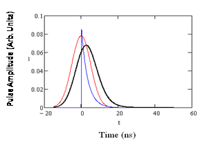
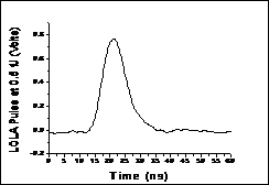
The variable offsets are mainly due to the impulse response of the detector electronics which distort the return pulse. As a result when the return energy changes the receiver pulses will be distorted and introduce a "range walk" or bias (sometimes referred to as “time walk”) that is a function of the received signal amplitude. The impulse response of the detectors may be modeled, to first order, by a simple RC lowpass filter. The convolution of a Gaussian pulse with the impulse response of an RC low pass filter is the error function. Figure 4‑1shows a simulation of a Gaussian pulse (red trace) with the impulse response of an exponential decay function from an RC filter (blue trace) and the resulting convolution (black trace) and Figure 4‑2 shows an actual pulse from the LOLA detector from subsystem testing. The impulse response of the detector will smear out any high frequency components in the laser pulse resulting in slightly wider pulsewidth and a ‘time-walk” as the energy and pulsewidth increase.

Since LOLA does not use a constant fraction discriminator we need to correct for this “range walk” which is dependent on the gain, threshold, and return pulse energy. The “range walk” correction due to the impulse response of all channels may be modeled in two different ways:

1. An empirical formula derived from test data that accounts for the pulse broadening and “time walk” effect based on the gain and threshold readback and the received energy.

2. A simple exponential (a lowpass RC filter with R=50 W and C = 68 pF) or a single-pole Butterworth filter based on the actual frequency response of the sub-system testing (see section 9.3).

Figure 4‑1 Convolution of Gaussian pulse with exponential decay function

Figure 4‑2 LOLA pulse at the output of the VGA

Both methods yield fairly good results but slightly different results. Currently we have developed calibration coefficients using the first method which give very good results. The results from a single-pole Butterworth filter were not as consistent.

In order to account for the variable offsets we define the following variables:

n = receiver channel number 1-5

thr_n = receiver threshold readback in millivolts

G_n = receiver gain readback (no units)

thr_s_n = thr_n/G_n

E_n = receiver energy in counts

em_n = minimum energy counts for channel n

EC_n = E_n - em_n

Define ratio R_n as follows:

The timing offset in nanoseconds (ln = natural log):

If EC > 0 :

If EC = 0:

Where S_n(G_n) and ∆_n(G_n) are 2^nd order polynomial functions of gain readback (G_n):

Coefficient for S_n = [s1, s2, s3] :

S₁=[-0.0006, 0.0336, -1.2694];

S₂=[-0.0006, 0.0396, -1.4347];

S₃=[-0.0006, 0.0343, -1.2236];

S₄=[-0.0006, 0.0330 ,-1.2144];

S₅=[-0.0006, 0.0341, -1.2523];

Coefficients for :

∆₁= [-0.00009, -0.0550, 20.28]

∆₂= [-0.00009, -0.0550, 20.28]

∆₃= [-0.00003, -0.0588, 18.46]

∆₄= [-0.00001, -0.0528, 16.61]

∆₅= [-0.00010, -0.0675, 18.47];

To compute time of flight range T_n in nanoseconds :

4.1.3 Zero Reference (Zero Range)

The range measurements are referenced to the front surface of the LOLA receiver lens. They can also be referenced to the LOLA cube. The distance between the LOLA receiver and the LOLA reference cube is cm 5.974 inches or 15.174 cm (Figure 4‑3).

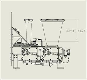
Figure 4‑3 LOLA reference cube distance from the receiver

The location of the LOLA cube is shown in Figure 4‑4.

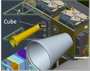
Figure 4‑4 LOLA Cube Location

The LOLA cube location (in cm) in the BCS coordinate system is

X = 172.906 cm

Y = 96.087 cm

Z = 52.301 cm

and is shown in Figure 4‑5 blow.

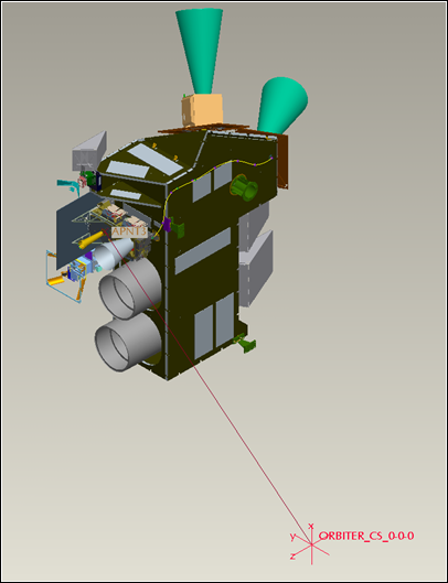
Figure 4‑5 Location of LOLA cube in BCS coordinate system

5.0 PULSEWIDTH CALIBRATION

5.1 TRANSMITTER PULSEWIDTH

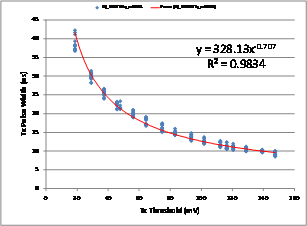
LOLA monitors the laser-pulse energy and the pulse width at threshold crossing, which may be used to infer the transmitted laser-pulse shape. Note that the pulse shape output from the LOLA SPOT 4 detector is the convolution of the actual pulse shape and the impulse response of the transmit energy monitor. (The nominal rise time for the SPOT4 detector is 3 ns). The relationship between the LOLA measured pulse width and the threshold value for laser 1 and 2 was measured and the result is given in Figure 5‑1 and Figure 5‑2. The nominal transmit threshold setting is 116 mV. The average transmitted laser-pulse energy is not expected to decrease significantly over the mission lifetime, thus the threshold value for the transmitted pulse should not have to be adjusted. If the laser or the transmitter common optics were to degrade, the threshold could be lowered to continue detecting transmitted laser pulses. There is approximately a factor of six adjustment that can be made on the transmit threshold (from 19 to 116 mV).


Figure 5‑1 Laser 1 Tx pulse threshold sweep	Figure 5‑2 Laser 2 Tx pulse threshold sweep

5.2 RECEIVER PULSEWIDTH

The received echo pulse width can be used to estimate the surface slope and roughness within the laser footprint. The received pulse width needs to be corrected for the fixed and variable time offsets just like the TOF. The same equations that are used to correct the TOF must be applied to the pulse width estimates.

The performance of the LOLA pulse width measurement (standard deviation) as a function of received energy is shown in Figure 5‑3. The error, as measured by the standard deviation, remains below 800 ps over all energies.

Figure 5‑4 shows the pulse width measurement from the nominal up to 6 to 25 ns vs the expected test pulse width (blue curve) and the corresponding residual ( red curve). The residual remains below 1 ns at all pulse widths.

Figure 5‑5 shows the pulse width measurement from the 25 to 50 ns vs the expected test pulse width (blue curve) and the corresponding residual ( red curve). The residual remains below 1 ns at all pulse widths.

Figure 5‑3 Received pulse width vs energy standard deviation

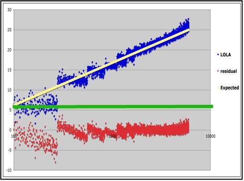
Figure 5‑4 LOLA Pulse width vs. Test pulse width for 6 to 25 ns

Figure 5‑5 LOLA Pulse width vs. Test pulse width for 25 to 50 ns

6.0 ENERGY CALIBRATION

6.1 TRANSMITTER ENERGY CALIBRATION

6.1.1 Precision

The LOLA transmitter has an on-board laser energy sensor (detector), which also serves as the fire acquisition detector. The detector is commonly referred as the SPOT4 or Transmit energy (Tx Energy) monitor. The transmit energy monitor was correlated with measurements made with an external energy meter to assess its performance at the system level (Figure 6‑1).

By correlating and normalizing the Tx Energy monitor with the external energy monitor (to normalize out any laser fluctuations) we determined that we can measure the transmitted energy with 1.3 % accuracy. There was no degradation in the precision performance of the Tx Energy monitor as a function of temperature. Using data for laser 1 in the hot and cold plateaus during instrument TVAC we determined that in the hot case the precision was 0.5%-1% and in the cold case it was approximately 1.0%. Thus, we expect the Tx energy precision requirement of 2% to be met at all temperatures even if the actual energy has changed considerably. The precision of the Tx Energy monitor measurement does not imply that it measures the laser energy with 2% absolute accuracy.

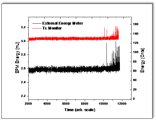
Figure 6‑1 Transmit energy calibration

6.1.2 Counts to Energy Calibration:

The equation that converts Tx Energy monitor from counts to laser energy is given below:

The equation was obtained using ambient temperature data (where the full energy of the laser beam could easily be measured) and it is an approximation from averaging different data sets.

The responsivity of the (Tx Energy) monitor changes significantly as a function of temperature, therefore a temperature correction must be applied to the equation above. The temperature correction was derived from the breadboard laser test data.

where T₀ is the energy at room temperature (T_room = 23.2 ^oC) and the T is the temperature of the SPOT4 detector. Unfortunately, there is no temperature sensor on the SPOT4 detector itself. However, the detector follows the laser bench temperature and the LEA electronics (with some lag). It does not get as cold as the laser bench temperature or as hot as the LEA electronics. The average of the two temperatures (laser bench and LEA electronics) should provide a reasonable approximation of the SPOT4 temperature.

(Note: Since there was no sub-system TVAC test of the flight transmitter the temperature dependence for the SPOT4 was derived from the breadboard laser test data and the EM laser TVAC data. At system level TVAC there was a fiber-optic pick-off for laser energy measurements which, unfortunately, showed large variations due to fiber optic coupling and transmission changes as a function of temperature and could not be used to derive the temperature correction).

6.2 RECEIVER ENERGY CALIBRATION

6.2.1 Precision

Each LOLA detector has an energy monitor circuit that estimates the received energy (Rx Energy) incident on each detector. The received energy per pulse is a direct measure of the lunar surface reflectivity and is given by [Gardner 1992]:

where E_Rx is the received energy, E_Tx is the transmitter energy, e_Rx is the efficiency of the receiver optics (from the telescope to the detector active area), A_Rx is the receiver aperture area, r is the surface reflectivity and r is the range to the target (lunar surface). By normalizing the received energy to the transmitter energy and knowing the range, we can determine the surface reflectivity of the lunar surface.

The energy monitor is essentially a peak sample and hold circuit with an integrator. The energy monitor circuitry is after the variable gain amplifier (VGA) and voltage buffer but before the timing circuit, which means it is affected only by the gain setting but not the threshold setting. The circuit is optimized for detection of energies from 0.1 to 3.0 fJ.

The specification for the energy monitor precision is to measure the relative energy within 12% from 0.1 to 3.0 fJ. This specification is met for energies above 0.2 fJ. At 0.1 fJ the precision can can be as large as 30% depending on which detector is used and its temperature.

An example of the Rx energy monitor precision as a function of the incident energy for detector 2 (D2) is shown in Figure 6‑2. The different plots show the precision at various temperatures during the system level TVAC test. The temperature in degrees C is listed in the graph legend. The laser used in the test is also shown in the graph legend (L1 and L2). The rest of the legend shows the date the test was performed. The precision is determined as the standard deviation divided by the mean value. Some variation in the energy calibration of the Ground Support Equipment is expected but from the plots it is clear that the 12% requirement (indicated by the light magenta dashed line) is met for all energies > 0.1 fJ but not at 0.1 fJ.

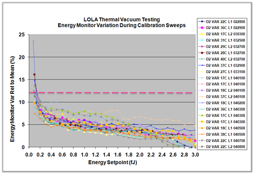
Figure 6‑2 Rx energy monitor for Detector 2.

(Legend explanation: The tests are all for detector 2 listed as D2 in the legend. The detector temperature in degrees C is listed as 22C, 36C, 17C, etc. The laser used in the test is also listed in the graph legend as L1 and L2. The rest of the legend shows the date the test was performe, e.g 022808 (is February 28 2008).

Tables Table 6‑1 through

Table 6‑3 show a summary of the precision of the energy monitor at three selected energy values: 0.1, 0.5, and 1.0 fJ for low (<20 ^oC), nominal (20-30 ^oC) and high (>30 ^oC). At higher energies, the energy monitor signal to noise ratio is increased the precision increases.

Table 6‑1 Energy Monitor Precision (in %) at 0.1 fJ

	Laser 1	Laser 1	Laser 1	Laser 2	Laser 2	Laser 2
	<20°C	20-30°C	>30°C	<20°C	20-30°C	>30°C
D1	12.5	15.1	15.1	15.2	15.8	18.5
D2	10.8	11.9	13.8	12.4	13.6	12.5
D3	14.5	14.3	13.7	19.3	16.8	14.4
D4*	11.0	12.1	13.9	13.9	14.0	9.9
D5	12.4	16.5	15.0	14.9	16.6	12.1

Table 6‑2 Energy Monitor Precision at 0.5 fJ

	Laser 1	Laser 1	Laser 1	Laser 2	Laser 2	Laser 2
	<20°C	20-30°C	>30°C	<20°C	20-30°C	>30°C
D1	7.0	5.9	6.3	6.3	7.2	6.4
D2	7.2	5.9	6.0	6.4	7.3	6.3
D3	8.1	6.3	6.4	7.3	7.7	7.1
D4*	7.0	5.4	5.9	6.7	7.6	6.1
D5	6.7	5.8	6.1	6.6	7.7	6.5

Table 6‑3 Energy Monitor Precision at 1.0 fJ

	Laser 1	Laser 1	Laser 1	Laser 2	Laser 2	Laser 2
	<20°C	20-30°C	>30°C	<20°C	20-30°C	>30°C
D1	5.81	4.71	5.61	5.73	6.08	5.68
D2	5.82	4.34	5.23	5.13	6.17	5.70
D3	6.00	4.96	5.03	5.46	6.17	5.64
D4*	5.66	4.42	4.62	5.31	5.90	5.26
D5	5.51	5.19	5.15	5.24	6.62	5.71

*The Rx energy monitor in detector 4 fails to measure the energy of a considerable number of pulses (the percentage of “missed” energy values can be as high as 25% depending on the energy). The “missed” pulses were excluded in the precision calculations shown in these tables.

6.2.1.1 Impact on Ice Detection

The possible detection of surface ice by LOLA, although not the instrument’s prime measurement, is considered a potential high-priority measurement to address one of LRO’s mission objectives.

The Rx energy monitor, normalized by the Tx energy monitor, is proportional to the surface reflectance at the laser wavelength. The reflectance of ice crystals on the lunar surface is expected to be approximately 4 times the reflectance of the regolith. The Rx Energy monitor meets and surpasses the 12% precision specification at energies > 0.1 fJ but does not meet it at the 0.1 fJ (nominal energy). Figure 6‑3 and Figure 6‑4 show the impact of the higher than 12% error at 0.1 fJ. Figure 6‑3 shows the ratio of the Received to the Transmit energy for regolith (RatioReg) with an albedo of 0.2 and the same ratio for regolith mixed with 4% ice (RatioIce) with an ice albedo of 0.8 as a function of the spot number or index on the ground (equivalent to distance). The large, connected points on the plots show a 10 point average of the corresponding ratios.

The assumption for this simulation was that the Tx energy monitor precision was 2% (which is met at all temperatures) and the Rx energy monitor precision was 10% (which is met at 0.2 fJ and higher). Poisson noise was used in the simulation.

A clear change in the energy ratio (proportional to the surface reflectivity) is visible between the regolith and the regolith mixed with ice. The change is of course, more pronounced if we average 10 spots. Figure 6‑4 shows the same ratios with the assumption that the Tx energy monitor precision was 2% and the Rx energy monitor precision was 20% (which is met at 0.1 fJ). The change in the energy ratio (proportional to the surface reflectivity) between the regolith and the regolith mixed with ice is now less visible but still possible to discern. The change is of course, more pronounced if we average 10 or more spots.

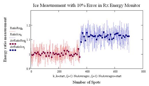
Figure 6‑3 Ice detection with 10% error in the Rx energy monitor

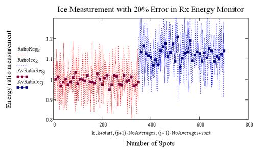
Figure 6‑4 Ice detection with 20% error in the Rx energy monitor

6.2.2 Counts to Energy Conversion

The energy monitor was characterized at sub-system testing and system level integration. The energy monitor is, to a first approximation, linear with energy, but has a gain dependent slope and offset. The following equations can be used to convert counts to energy, E, (in fJ):

where, slope(G) and offset(G) are the gain dependent slope and offset. The equation that describes the gain dependent slope is given by:

The offset is best described by a quadratic fit (although a linear fit also gives adequate results).

Gain in the equations above is the gain read back.

Table below gives the coefficient values for all 5 detectors. These equations are valid for energies ≥ 0.2 fJ. At 0.1 fJ the equations do not give a very accurate energy value. Note that in this case are the raw counts out of the energy monitor without any offsets subtracted.

Table 6‑4 Energy monitor counts to energy calibration

		Slope Coefficients			Offset Coefficients
	A	B	C	A	B	C
Detector 1	0.00914	0.07437	13.4092	-0.84429	0.03313	-0.00032235
Detector 2	0.00829	0.07399	12.9082	-0.82769	0.03376	-0.00034980
Detector 3	0.01103	0.0813	11.44682	-0.63522	0.02518	-0.00025046
Detector 4	0.00985	0.08125	11.10461	-0.8598	0.03452	-0.00033139
Detector 5	0.00852	0.06865	14.19706	-0.74418	0.02174	-0.00010699

Note that absolute energy accuracy of Rx energy monitor (i.e. the counts to fJ conversion) is no better than 20-30% (after all LOLA is not an absolutely calibrated radiometer but an altimeter). However, the relative energy values (in counts) will remain within the specification of 12% except at the lower energies (0.1 fJ) as indicated above.

6.2.3 VGA, Digitizer and Energy Monitor Saturation

The counts to energy equations are only valid in the linear, non-saturation regime for the digitizer and the amplifier chain. The LOLA digitizer that converts the energy monitor voltage into counts is an 8-bit digitizer. The maximum number of counts that the digitizer can output is 255 counts. Any value greater than 250 is very close to the digitizer saturation regime.

In addition to the digitizer the VGA/buffer amplifier chain can saturate depending on the gain setting of the amplifier chain. Figure 6‑5 and Figure 6‑6 show data from subsystem testing (flight spare detector) below and above the VGA saturation and the corresponding Rx energy monitor response for different gains, G. The maximum output voltage for the amplifier chain is approximately 2.0-2.1 Volts. This corresponds to approximately 1.3 fJ assuming a responsivity of 310 V/W, full gain, and a 9.2 ns pulse (test parameters for Figure 6‑5 and Figure 6‑6).

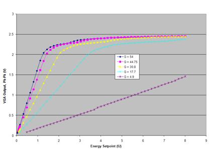
Figure 6‑5 VGA pulse peak-peak voltage vs. energy for various gain settings

Figure 6‑6 Rx energy monitor voltage vs. energy for various gain settings

7.0 TRANSMITTER CALIBRATION

7.1 LASER FAR FIELD PATTERN

The laser far field pattern was measured at the subsystem (laser) level with a 4-m focal length off-axis parabola collimator and a CCD camera at the focal point. The data were analyzed using commercial beam analysis software (BeamView^© by Coherent). The laser beam profiles after the beam expander integration are show in Figure 7‑1and Figure 7‑2.

Figure 7‑1 Laser 1 profile with CCD at simulated vacuum Focus (18 mm from OAP focal plane)

Figure 7‑2Laser 2 profile with CCD at simulated vacuum Focus (18 mm from OAP focal plane)

The laser divergence prior to the beam expander integration was:

• Laser 1

• FF Divergence 1.76 mrad (= 97.8 urad after ×18 beam expander)

• 99% energy enclosed within aperture diameter of 5.7 mm - 1.6 × 1/e² dia, or

< 1 % of energy lies outside of 2 x 1/e² diam.

• Circularity = 0.91

• Laser 2

• FF Divergence 1.72 mrad (= 95.6 urad after ×18 beam expander)

• 99% energy enclosed within aperture diameter of 5.7 mm - 1.7 × 1/e² dia, or< 1 % of energy lies outside of 2 x 1/e² diam.

• Circularity = 0.97

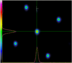
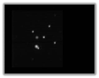
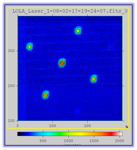
During system level environmental testing the laser far field pattern was measured using an off-axis parabola and a different CCD camera. The data were analyzed using custom-developed software that fit the laser images to a two-dimensional Gaussian surface. A sample of laser images (along with reference cubes images and a fiduciary image) are show in Figure 7‑3 and Figure 7‑4.

Figure 7‑3 Black and white CCD image showing 5 laser spots, two reference cubes and one fiduciary spot during TVAC.

Figure 7‑4 False color image of 5-spot laser beam pattern without reference cubes or fiduciary.

7.2 TRANSMIT PATH EFFICIENCY

The transmit optical path efficiency of LOLA (beam expander and DOE) was measured to be 78%. However, the five spots are not equal in energy. The center spot has most of the energy, 21.8 % of the total energy, with the other spots having 14.1, 12.9, 15.0 and 14.3 %, for channels 2, 3, 4, and 5 respectively, of the total energy. The ratio is an artifact of the Diffractive Optical Element (DOE) but it proves beneficial since the center spot (i.e. the center detector) is the detector that has the laser ranging channel and is exposed to much higher background solar power (up to 5-8 nW for a full sun-lit earth) than the other four detectors, which only look at the lunar background. The separation between the spots varies from 502 to 513 mrad.

7.3 LASER DIVERGENCE

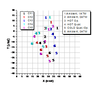
The laser far field pattern remained nearly TEM₀₀ mode over the entire operating temperature range. The divergence was calculated as the average of the x and y Gaussian 1/e² widths (Figure 7‑5). The laser divergence and circularity (defined as the Ratio of Major to Minor Axes, in this case, the Ratio of the x and y Gaussian widths obtained by the fit) as a function of temperature are shown in Table 7‑1. (At ambient pressure the transmitter optics is out of focus which results in high divergence).

Table 7‑1 Laser Divergence

	Laser 1 (urad)	Circularity	Laser 2 (urad)	Circularity
Ambient 1 Atm	153.1	Out of focus	147.9	Out of focus
Ambient 0ATM (Start)	100.0	1.08	94. 9	1.19
Hot Qual.	106.7	0.96	97. 5	1.18
Cold Qual/Op.	103.6	1.30	110.7	1.24
Hot Operational	104. 5	1.29	102.5	1.17
Ambient 0 Atm (End)	109.9	1.14	101.7	1.30

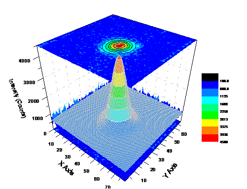
Figure 7‑5 Laser Profile of Channel 1

7.4 LASER POINTING JITTER

The laser pointing jitter was monitored at the sub-system level and also during the system level environmental testing.

Figure 7‑6 shows the pointing jitter at the subsystem level and Figure 7‑7shows the laser 1 pointing jitter after analyzing 450 images taken during the system level TVAC testing over al temperatures. The images were analyzed for the relative separation between the central laser spot and a reference cube. The jitter in both sub-system and system level environmental testing was approximately 5 mrad in the x and y direction.

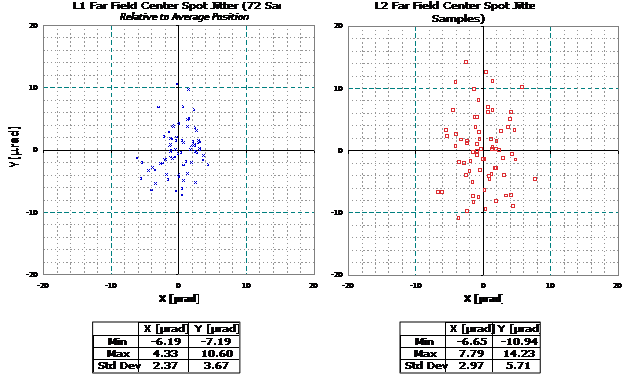
Figure 7‑6 Laser Pointing Jitter at sub-system level

Figure 7‑7 Laser Pointing Jitter at system level

7.5 LASER WAVELENGTH

The laser wavelength as measured at the sub-system delivery (see Laser IDR) was 1064.4 nm. During system level environmental testing the laser wavelength was monitored by a wavemeter (operating in CW mode). The wavelength change as a function of laser bench temperature for laser 1 and laser 2 are shown in Figure 7‑8 and Figure 7‑9. The overall change in the laser wavelength is ~ 0.1-0.13 nm. The discontinuous changes in the laser wavelength are 0.04 - 0.05 nm. To first order the change in wavelength (without the discontinuous changes) is ~ 0.06-0.07 nm/deg C.

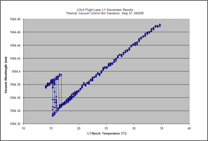
Figure 7‑8 Laser 1 Wavelength over Temperature

Figure 7‑9 Laser 2 Wavelength over Temperature

The discontinuous changes in the wavelength could be due to changes in the mode structure of the laser and/or the wavemeter operation, which will report the wavelength of only the most dominant mode.

The laser wavelength did not change after shipment to the launch site. It was measured again at the launch facility (Astrotech) – see Figure 7‑10.

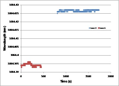
Figure 7‑10 Laser Wavelength at Astrotech

7.6 LASER ENERGY

The laser energy at room temperature at the time of sub-system delivery was ~ 2.6 mJ for laser 1 and ~ 3.0 mJ for laser 2 after the beam expander. This was verified at the system level prior to laser integration onto the instrument. The laser energy was measured again at the orbiter level (with a different energy meter). The energy for laser 1 was 2.66 mJ, and 3.22 mJ for laser 2. The difference between sub-system and system measurements is probably due to the calibration of the energy sensors - the absolute calibration for each meter is 10%. No degradation of the laser energy was observed from delivery to orbiter integration.

The laser energy varies as a function of temperature. The dependence of the laser energy on the temperature was monitored at the sub-system level in air which is not representative of the flight configuration. The EM laser was tested in vacuum and its temperature dependence is more representative of the flight configuration. Ultimately, the laser energy (Tx) can be estimated from the Tx energy monitor from the equations in Section 6.1.2. Both lasers exhibited hysteresis when the temperature was cycled.

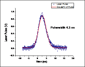
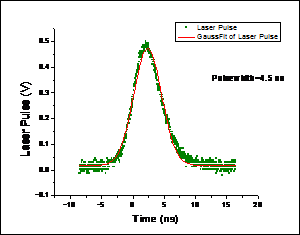
7.7 LASER PULSE SHAPE AND MODE-BEATING

The laser-pulse shape was measured at sub-system (laser) integration using a high-speed photo detector and oscilloscope, and during system environmental testing. The sub-system results are shown in Figure 7‑11. The pulse width varies from 4.3 to 4.9 ns full width at half maximum (FWHM). Sample waveforms from the system level environmental test measured by a high speed detector are shown in Figure 7‑12 and Figure 7‑13. The pulsewidth was the same as the sub-system measurements (within the experimental error).

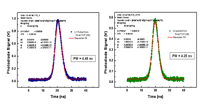
Figure 7‑11 Laser Pulse width at sub-system level

Figure 7‑12 Laser 1 Pulse width

Figure 7‑13 Laser 2 Pulse width

The LOLA laser is not a single mode laser. It will occasionally operate in more than one mode and those modes may beat against each other producing a series of very short pulses. Several examples of mode beating pulses are shown in Figure 7‑14. The pulses were recorded by an external high speed photodiode and oscilloscope during instrument level TVAC testing.

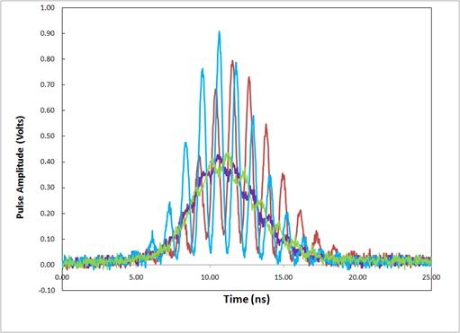
Figure 7‑14 Laser Mode beating example

The impulse response of the transmit energy monitor will “smear out” the short mode-beating pulses. Laser 1 rarely exhibits multi-mode behavior (1-2 % of the total number of shots in steady state), whereas laser 2 exhibits multi-mode behavior much more frequently (can be ~ 25% of the time). The multi-mode behavior is also dependent on the laser temperature. The transmit energy monitor can be used to detect the multi-mode behavior of the laser since the peak energy shows a large increase. Thus the Tx energy monitor should be used to flag the returns for the distorted laser pulse shapes.

8.0 RECEIVER CALIBRATION

8.1 RECEIVER ALIGNMENT AND BORESIGHT

The receiver field of view (FOV) was verified prior to instrument integration and was found to be 400 ± 20 μrad (FWHM) for all 5 channels (see Figure 8‑1). The channel to channel spacing was 500 ± 20 μrad.

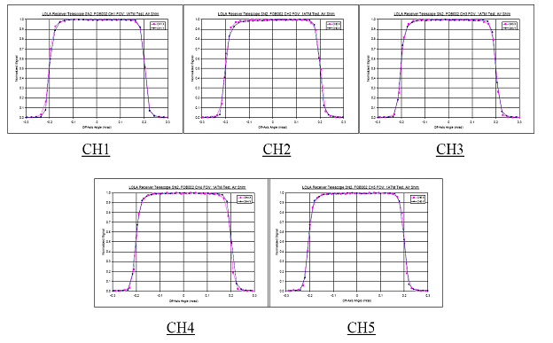
Figure 8‑1 Receiver Field of View

The FOV was also verified during instrument environmental testing by back-illuminating the LOLA detectors through the test ports with a 1061 nm diode laser. The shorter wavelength was chosen to minimize the amount of power on the detectors but it resulted in some image degradation since the image at 1061 nm was slightly defocused. In the hot case (a DT of +15 ^oC of the receiver), some degradation of the FOV (~ 10-20 mrad) was observed due to the defocus of the receiver telescope bulk temperature change and the laser diode wavelength (1061 vs. 1064 nm). For the cold case (a DT of -7 ^oC) no significant change in FOV was observed. From these results, the FOV is expected to remain within its nominal range 400 ± 20 μrad (FWHM) for all 5 channels.

The channel spacing of 500 ± 20 μrad remained virtually unchanged during instrument environmental testing indicating very little temperature dependence of the DOE. Thus, on orbit we expect very little change in the beam separation.

The alignment of the receiver telescope to the transmitter was verified and tracked throughout the instrument I&T process using the back-illumination method and imaging the laser spot and the detectors’ FOV on a CCD using an off-axis parabola.

Table 8‑1 shows the boresight temperature dependence (shift) during instrument environmental testing. The data are also summarized pictorially in Figure 8‑2 through Figure 8‑5. For both laser 1 and laser 2 there is a small boresight shift as a function of temperature on the order of 30-45 urad mainly in the y direction.

Table 8‑1 Boresight Error during instrument TVAC

Figure 8‑2 Laser 1 Boresight during instrument TVAC

Figure 8‑3 Laser 1 Boresight during instrument TVAC (zoom)

Figure 8‑4 Laser 2 Boresight during instrument TVAC

Figure 8‑5 Laser 2 Boresight during instrument TVAC (zoom)

We monitored the boresight alignment through observatory I&T. At the observatory level a lateral transfer retro-reflector (LTR) and a pair of Risley prisms were used to test the boresight alignment. The boresight was also verified at the launch site (Astrotech). The boresight alignment summary for all 5 channels (RX1-5) is shown in Figure 8‑6. The shifts are below the original allocation for spacecraft I&T.

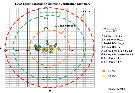
Figure 8‑6 Boresight summary

8.2 RECEIVER EFFICIENCY

The efficiency of the LOLA receiver components was measured at subsystem and verified at the system level. The telescope transmission was 99%. The aft optics and fiber transmission for each channel are show in Table 8‑2.

Table 8‑2Aft-optics and fiber transmission efficiency

Receiver Channel	Aft Optics Transmission %	Fiber Transmission %
1	86.1	98.6
2	90.4	97.7
3	87.5	98.5
4	94.2	96.8
5	87.3	93.5

8.3 DETECTOR GAIN, BANDWIDTH, RESPONSIVITY AND DARK NOISE

8.3.1 Gain Control

The LOLA detectors are silicon avalanche photodiodes (APD) packaged in a hermetically sealed package with an integrated transimpedance amplifier. The LOLA detector board amplifies the detector hybrid output. The amplification of the hybrid output is performed by a variable gain amplifier (VGA) and a fixed gain buffer with a gain of 5. The VGA gain is variable over a range of <0.5 to 10, controlled by an externally d.c. voltage generated by the DU. The gain dependence on the voltage (digitizer counts) for detectors 1-5 are given by the equations below:

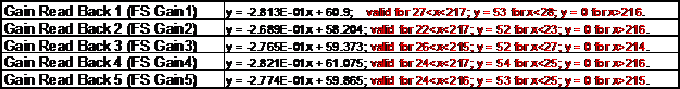
where y is the total gain (buffer x VGA) and x is the gain setting in counts.

After amplification a high speed comparator performs a discrimination function on the received pulse and provides the timing information to the Digital Unit. The threshold levels for the comparator are set by the DU and fed directly to the comparator input. The threshold voltage dependence on the digitizer counts for detectors 1-5 are given by the equations below:

Similarly the threshold voltage dependence on the digitizer counts for the SPOT4 (transmit) detectors is given by the equation below:

where y is the threshold voltage in mV and x is the threshold setting in counts.

8.3.2 Detector Responsivity

The overall receiver responsivity (in Volts/W) at the comparator input as a function of the optical signal onto the APD can be expressed as

where η_APD is the APD quantum efficiency, G_APD is the APD gain which includes the photoelectron multiplication and the gain of transimpedance gain of the hybrid, G_Bufferis the voltage gain of the buffer amplifier, and G_VGA is the VGA voltage gain.

Only the products of and can be measured at the sub-system level. The values were measured at the sub-system level and are shown in Table TBD below.

Detector	(× 10⁵ V/W) ± 20%
1	3.1
2	3.4
3	3.1
4	3.4
5	3.2

The pulse waveform in volts at the comparator can be approximated as the convolution of the received optical signal pulse shape with the receiver impulse response of each detector channel considered. The output of the comparator can be determined by comparing the pulse waveform with the threshold level. The commanded and read back threshold settings for each of the channels are found in the telemetry.

8.4 DETECTOR BANDWIDTH

The detector bandwidth (3 db point) was measured at the sub system level for all five detectors. The bandwidth for all five detectors is approximately 46 ± 5 MHz. Figure 8‑7 shows the frequency response of detector 2 at different gain settings with no light impinging on the detector. The bandwidths for all detectors five is shown in Table 8‑3.

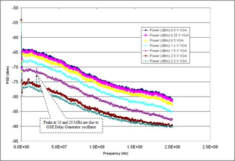
Figure 8‑7 Detector Bandwidth

Table 8‑3 Detector Bandwidths

*Detector Board SN*	*Bandwidth* ± 5 (MHz)
SN001	44.1
SN002	46.5
SN003	47.5
SN004	49.0
SN005	44.1

8.5 DETECTOR DARK NOISE, PROBABILITY OF DETECTION AND NOISE COUNTS

The receiver dark noise, i.e., the noise with no light onto the detector, was measured to be 9 nV/√Hz (in a 1 Hz bandwidth) at the maximum VGA gain setting. The noise level was obtained at the sub-system (detector) level and compared favorably with the manufacturer’s value of 12 nV/√Hz. The noise of the detector was deduced assuming the VGA noise was 6.0 nV/√Hz at maximum gain, and the buffer noise is 3.0 nV/√Hz (per manufacture’s specifications). These values translate to an overall noise level of approximately 3.9 mV rms at the output of the detector-amplifier chain at maximum gain and a bandwidth of 46 MHz.

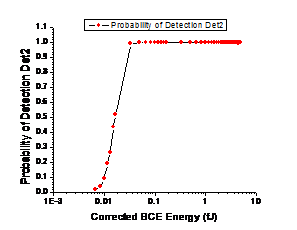
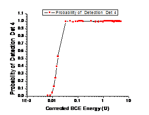
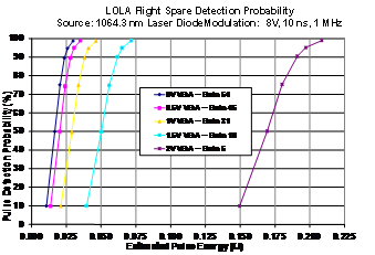
The noise level will translate to minimum detectable pulse energy for the altimeter at approximately 0.01-0.03 fJ (corresponding to ~ 95-165 km), albeit with a reduced probability of detection. The probability of detection was measured at the system and sub-system level. At the system level all five detectors were tested by varying the energy into the receiver (Figure 8‑8 through Figure 8‑12). The probability of detection is affected by the amount of background light. The lunar background levels are low (typically less than 800 pW including stray light) and are not expected to impact the probability of detection. However, the LR detector (detector 1), when the LR telescope is looking at the earth, is expected to see a significant amount of background light (up to 7 nW for a sunlit earth). The high background levels will reduce the probability of detection. This was expected and was a known trade-off in the design when the LR system was designed and accepted. The probability of detection as a function of energy for different gain settings was also measured for the flight spare detector (Figure 8‑13).

Figure 8‑8 Detector 1 Probability of Detection

Figure 8‑9 Detector 2 Probability of Detection

Figure 8‑10 Detector 3 Probability of Detection

Figure 8‑11 Detector 4 Probability of Detection

Figure 8‑12 Detector 5 Probability of Detection

Figure 8‑13 Flight Spare Detector Probability of Detection

8.5.1 Noise Counts

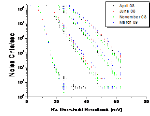
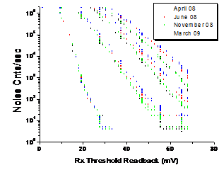
The LOLA receiver noise counts (or false-alarm rates) were measured as a function of the threshold levels for each detector during both the detector assembly level test and instrument environmental tests. The noise counter readings are very sensitive to the receiver noise levels and can be used as an indicator of the receiver dark noise and responsivity to background light.

Figure 8‑14 through Figure 8‑18 show the false-alarm rates vs. threshold level under dark-noise (0 nW), 1, 3, and 5 nW for all channels for Gain 50 for selected days (instrument post-TVAC, observatory and at the launch site). Some variation should be expected because of the test setup and calibration of the test source, but overall the noise counts have remained fairly consistent over time.

Figure 8‑14 Detector 1 Noise Counts

Figure 8‑15 Detector 2 Noise Counts

Figure 8‑16 Detector 3 Noise Counts

Figure 8‑17 Detector 4 Noise Counts

Figure 8‑18 Detector 5 Noise Counts

8.6 ENERGY RESET GLITCH

The Rx energy monitor uses an energy reset pulse to reset the integrator and peak sample and hold circuitry. Unfortunately the energy reset causes a glitch in the output of the amplifier chain and a subsequent glitch in the timing output (Figure 8‑19) if it rises above the threshold setting. Depending on the received pulse amplitude more than one threshold crossing may be detected and subsequently more than one timing glitch may be present. The glitch occurs when the energy reset changes, approximately 60 ns and ~ 33 ms after the received pulse. (For clarity, only the first glitch at 60-80 ns is shown in Figure 8‑19).

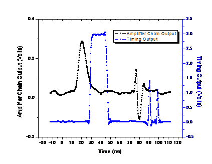
Figure 8‑19 Energy Reset Glitch

The glitch produces additional noise counts and has an impact on the algorithms. We were unable to rectify this problem in hardware before integration due to design and schedule constraints. However, the algorithm team was successful in implementing a fix which is described in detail in the algorithm document.

8.7 DETECTOR TEMPERATURE DEPENDENCE

All five detectors were tested at the sub system level but only one underwent temperature cycling in order to accommodate the flight schedule. The results of the temperature cycling for flight detector 3 are shown in Figure 8‑20 and Figure 8‑21 The dark noise counts increase as a function of temperature. The polynomial that describes the dark noise increase is given in the graph (where x=Temperature). When light impinges on the detector the response is different. The combined temperature dependence of silicon and the internal detector hybrid electronics show a decrease in the noise counts as a function of temperature (Figure 8‑21).

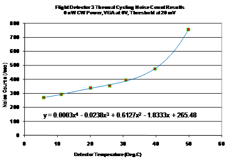
Figure 8‑20 Dark noise counts as a function of temperature

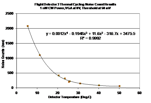
Figure 8‑21 Noise counts vs. temperature

9.0 ACKNOWLEDGEMENTS

We like to thank Dave E. Smith and Maria T. Zuber, the Principal Investigator and Deputy Principal Investigator of LOLA, for their unwavering support and leadership in the development of LOLA. We would also like to thank the entire LOLA instrument and Laser Ranging team from NASA Goddard Space Flight Center for their dedication and hard-work without whom none of this would have been possible.

10.0 REFERENCES

Abshire J.B., X. Sun, H. Riris, J. M. Sirota, J. F. McGarry, S. Palm, D. Yi, P. Liiva, "Geoscience Laser Altimeter System (GLAS) on the ICESat Mission: On-orbit measurement performance", Geophys. Res. Lett., 32, L21S02, doi:10.1029/2005 GL024028, 2005.

Gardner, C.S. IEEE TRANSACTIONS ON GEOSCIENCE AND REMOTE SENSING, Vol. 30, No. 5, Sept. 1992

Smith, D.E., M.T. Zuber, H.V. Frey, J.B. Garvin, J.W. Head, D.O. Muhleman, G.H. Pettengill, R.J. Phillips, S.C. Solomon, H.J. Zwally, W.B. Banerdt, T.C. Duxbury, M.P. Golombek, F.G. Lemoine, G.A. Neumann, D.D. Rowlands, O. Aharonson, P.G. Ford, A.B. Ivanov, P.J. McGovern, J.B. Abshire, R.S. Afzal, and X. Sun," Mars Orbiter Laser Altimeter (MOLA): Experiment summary after the first year of global mapping of Mars", J. Geophys. Res.,106, 689, 2001.

Zwally H.J., B. Schutz, W. Abdalati, J. Abshire, C. Bentley, A. Brenner, J. Bufton, J. Dezio, D. Hancock, D. Harding, T. Herring, B. Minster, K. Quinn, S. Palm, J. Spinhirne, R. Thomas, (2002), "ICESat’s laser measurements of polar ice, atmosphere, ocean, and land", J. of Geodynamics, Special Issue on Laser Altimetry 34, 405, 2002.